Bayes' Ball Statistics
Thomas Bayes, An Essay Towards Solving a Problem in the Doctrine of Chances, opens with the following problem:
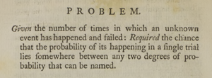
Given the number of times in which an unknown has happened and failed: Required the chance that the probability of its happening in a single trial lies somewhere between any two degrees of probability that can be named.
Bayes took the uniform prior, that is, he assumed that any probability was as likely as any other. In our coin-flip adventure, we assumed there were only 11 evenly spaced possible values for the unknown probability \(p\), so we could simply say each value has a probability of \(1/11\) of being right. But Bayes considered the continuous distribution over \([0, 1],\) so each value is drawn with probability zero. How do we proceed?
The trick is to study ranges instead of point values. Using the language of geometry, Bayes defined the uniform prior by stating that a value in the interval \([a, b]\) is drawn with probability \(b - a.\) Similarly, he asked for the posterior probability that \(p\) lies within a given range.
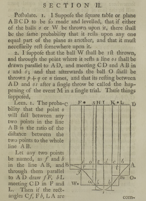
Bayes imagined throwing a ball on a table, whose landing position is as likely as any other (uniform prior) to represent drawing \(p\) uniformly from \([0,1]\). Next, he imagined repeatedly throwing a second ball on the table. A throw of this second ball counted as a happening when it landed to the right of the first ball.
We’ll say "success" instead of "happening", and in our demo above, we define the left side to be a success so that higher probabilities of success appear further to the right. (We can imagine we’re watching from the other side of Bayes' original table.)
For each \(p\), the probability of observing \(m\) successes out of \(m + n\) trials is:
\[ f(p) = {m + n \choose n} p^m (1 - p)^n \]
Bayes drew a picture of the table, and along its bottom edge, plotted \( f(p) \) for \(p \in [0,1] \) for a specific albeit unspecified choice of \(m, n\). To modern eyes, the graph looks upside-down, and it seems we could do without the rest of the table; perhaps a side view would have been better.
In Proposition 9, Bayes solves the problem using what we now call the sum rule and the product rule. Bayes describes the product rule in Proposition 3:
\[ P(A|B) P(B) = P(AB) \]
Let \(A\) be the event that \(a < p < b.\) Let \(B\) be the event that \(m\) successes and \(n\) failures have been observed. By the sum rule, and a dash of calculus, we find \(P(AB)\) is the area under the curve \(f\) between \(a\) and \(b\). Similarly, we find \(P(B)\) is the area under the curve \(f\) between \(0\) and \(1\).
Thus \(P(A|B),\) the probability that \(a < p < b\) given that there have been \(m\) successes and \(n\) failures, is their ratio. In modern notation:
\[ P(a < p < b | m, n) = \frac{ \displaystyle \int_a^b p^m (1 - p)^n dp }{ \displaystyle \int_0^1 p^m (1 - p)^n dp } \]
The binomial coefficient \({m + n \choose n} \) cancels out.
Bayes knocked it out of the park. For example, if we flip a coin 20 times and see heads 12 times, we now know how to compute the probability that \(0.45 < p < 0.55:\)
jsEval "curl_module('../haskell/GenFun.ob')"
import GenFun

evalPs x = foldrPs (\a b -> a + x*b) 0

f = int $ (x 1)^12 * (1 - x 1)^8

(evalPs 0.55 f - evalPs 0.45 f) / (evalPs 1 f - evalPs 0 f)
The uniform prior forecasts a 10% chance of \(p \in (0.45, 0.55)\), and observing 12 heads out of 20 flips updates this probability to over 25%.
One can quibble about the uniform prior. Indeed, if handed a coin that looks and feels fair, I might use a prior weighted heavily at 0.5 with rapidly shrinking tails on either side. But firstly, in this problem, unless our prior is egregiously unbalanced, we ultimately reach similar conclusions.
Secondly, and more importantly, Bayes showed how to go from first principles to an ironclad conclusion, which my frequentist undergraduate course in probability and statistics was unable to do.
Beta version
It turns out that the above denominator is an integral that was studied by Euler and Legendre. Binet named it the beta function:
\[ \unicode{x392}(z_1, z_2) = \int_0^1 t^{z_1-1}(1-t)^{z_2-1} dt \]
for all \(z_1, z_2 \in \mathbb{C}\) such that \(\Re(z_1), \Re(z_2) > 0.\) (Its symbol is an uppercase beta and not a Latin B, which you can probably only tell by looking at the unicode.)
Because of this, we say the probability density function:
\[ f(p) = \frac{ \displaystyle p^m (1 - p)^n dp }{ \displaystyle \int_0^1 p^m (1 - p)^n dp } \]
is the beta distribution parameterized by \((m + 1, n + 1);\) Proposition 9 says \( P(a < p < b | m, n) = \int_a^b f(p) dp. \) See if you can spot other beta distributions below.
Bayes versus Bernoulli
In Proposition 5, Bayes notes the product rule is symmetric:
\[ P(B|A) P(A) = P(AB) \]
which implies what we now call Bayes' theorem:
\[ P(A|B) = \frac{P(B|A) P(A)}{P(B)} \]
While Bayes had no need for Bayes' theorem to solve his problem, the underlying idea is the same. We want \(P(A|B),\) but computing it directly is difficult. Bayes' insight was to calculate it indirectly, via probabilities that we know how to compute.
Perhaps this seems like elementary algebra today, but when the brilliant mathematician Jacob Bernoulli faced the same problem, loosely speaking, he argued that \(P(B|A)\) was close enough to \(P(A|B),\) so he had no need to compute anything else. This famous mistake is known as Bernoulli’s fallacy (Clayton), Bernoulli’s swindle (Diaconis and Skyrms), Bayesian wishful thinking, or inverse probability error. (Bernoulli’s own term was certa moraliter: morally certain.)
To be fair, Bernoulli was a pioneer in a area of mathematics that was in its infancy, and for the problems that he studied, such as urns containing black and white pebbles, the difference is small.
However, today’s orthodox statisticians, or frequentists, have no excuses to continue building upon Bernoulli’s error, especially since the difference matters a great deal for the problems they study. Frequentism has led to new names for the original sin, such as the prosecutor’s fallacy and base rate neglect, which hint at tragedies caused by their methods. And it has led to questionable science, for example, according to frequentism, college students have extra-sensory perception, but only when thinking about erotic images (Bem 2011).
Bayes and Means
Bayes already beats generations of frequentists at their own game, but let’s add insult to injury by predicting the future. After \(m\) successes and \(n\) failures of a repeated experiment, what is the probability the next experiment will succeed?
Let’s pick an example. We flip the coin 20 times and see head 12 times. What is the probability the next flip is heads?
Frequentists say the "best estimator" of the true probability is simply the mean number of successes: 12/20. But they never say why. Mackay: "there is no clear principle for deciding which criterion to use to measure the performance of an estimator; nor, for most criteria, is there any systematic procedure for the construction of optimal estimators." Clayton goes further:
Considering the names of all the various properties of estimators and tests in the statistical literature, it’s hard not to notice that they all seem to embed value judgments, suggesting that this particular estimator or test is good. We have already mentioned unbiased and consistent estimators. There are also efficient estimators, admissible estimators, dominant estimators, robust estimators, uniformly most powerful tests, and, surely the best example, the best linear unbiased estimator. It seems nearly certain that all this normativity is a by-product of the political infighting and jockeying for position between various camps within the world of frequentist statistics over the course of the last century. As different factions fought for legitimacy and for acceptance of their methods as standard, they must have thought it advantageous to give their methods virtuous-sounding names. Who would want to be seen as being in favor of bias, inconsistency, inefficiency, inadmissibility, subordination, frailty, powerlessness, or…worst-ness?
[The internecine squabbles mean that some frequentists may compute differently to how we portray them here. If so, then good! Inconsistencies further expose frequentism’s unprincipled nature. Also, the only thing each faction hates more than each other is Bayesian reasoning, so there is no danger of any of them being correct. Clayon: "Fisher, in particular, was known to fly into a rage any time the topic of inverse probability was raised." We’re not actively straw-manning; it’s just that frequentism is already a set of mutually contradictory straw men.]
While the mean 12/20 is also the mode (the most likely value), why should this property imply predictive power? For instance, imagine in some problem we found 12/20 is the most likely value, but we also found slightly lower peaks at 18/20 and 19/20 with most of the probability mass nearby. Would you still want to go with 12/20?
I believe even non-technical people can understand the issue. Suppose one-third of adults finish high school but never finished college, one-quarter have an college degree, and one-quarter have a graduate degree. (The remainder never made it out of high school.) Should we predict that a randomly chosen adult only has a high school diploma?
This is Bayes' Ball
What would a Bayesian do? Why, use Bayes' theorem of course! Let \(h\) denote "the next flip is heads"; we seek \( P(h | 12, 8). \) By the sum rule:
\[ P(h | 12, 8) = \int_0^1 p P (p | 12, 8) dp \]
By Bayes' theorem:
\[ P(p | 12, 8) = \frac{P(12, 8 | p) P(p)}{P(12, 8)} \]
Now we tackle the factors on the right-hand side. We have:
\[ P(12,8|p) = {20 \choose 8} p^{12}(1-p)^8 \]
and by the sum rule:
\[ P(12,8) = \int_0^1 P(p) {20 \choose 8} p^{12}(1-p)^8 dp \]
As before, the continuous prior implies \(P(p) = 0\), an inconvenience which we handle in the same manner Bayes did: with ranges. By abuse of notation, for a continuous variable we use \(P()\) to denote a probability density. We tacitly promise to integrate eventually to recover a probability. See page 30 of Mackay. For the the uniform prior over the unit interval, the probability density is \(P(p) = 1\) for all \(p \in [0,1]. \)
\[ P(p|12,8) = \frac{ {20 \choose 8} p^{12}(1-p)^8 } { \int_0^1 {20 \choose 8} p^{12}(1-p)^8 dp } \]
Via integration by parts and mathematical induction:
\[ \int_0^1 p^m(1-p)^n dp = \frac{m! n!}{(m + n + 1)!} \]
Thus:
\[ \begin{align} P(h | 12, 8) &= \int_0^1 p P (p | 12, 8) dp \\ &= \frac{\int_0^1 p p^{12}(1-p)^8 dp} {\int_0^1 p^{12}(1-p)^8 dp} \\ &= \frac{12! 8! / 21!}{13!8!/22!} \\ &= \frac{13}{22} \end{align} \]
In brief, we arrive at Bayes' Proposition 9 except the numerator has an extra factor \(p\) and its limits are \(0\) and \(1\) instead of \(a\) and \(b\), which then results in a bunch of factorials that cancel each other out.
In general, assuming the uniform prior for \(p,\) if there have been \(m\) successes and \(n\) failures, the probability that the next trial is a success is:
\[ \frac{m + 1}{m + n + 2} \]
This was first discovered by Laplace, and known as the rule of succession, who worked independenty of Bayes along the same lines. (Later, he became aware of Bayes and praised him.)
To recap, from first principles, we have derived the unique prediction that logically follows from our assumptions.
We build the demo at the top of the page showing it off:
parseFrac = uncurry (/) . foldl (\(a, b) d
  -> (a*10 + fromIntegral (ord d - ord '0'), b*10)) (0.0, 1)
jsrandom = parseFrac . drop 2 <$> jsEval "Math.random()"
play = do
  jsEval_ "play.disabled = true; onemore.disabled = true;"
  jsEval_ "bayestable.innerHTML = \"<rect x='0' y='-0.1' width='1' height='0.2' stroke-width='0.005' stroke='black' fill='none' />\";"
  unknownBall <- jsrandom
  jsEval_ $ "bayestable.innerHTML += \"<circle cx='" ++ show unknownBall ++ "' cy='0' r='0.07' fill='yellow' stroke-width='0.002' stroke='black' />\";"
  let
    colorBool True = "green"
    colorBool False = "red"
    update m n = do
      let
        ps = [(p, p^m * (1-p)^n) | p <- [0,0.01..1]]
        sup = foldr1 max $ snd <$> ps
        ps' = unwords [show x ++ "," ++ show ((sup - y) / sup) | (x, y) <- ps]
      jsEval_ $ "bayesgraph.innerHTML = \"<polyline points='" ++ ps' ++ "' fill='none' stroke='black' stroke-width='0.001' />\";"
      let
        status = unlines
          [ "successes (m) = " ++ show m
          , "failures (n) = " ++ show n
          , "probability of success by the rule of succession = " ++ show (fromIntegral (m + 1) / fromIntegral (m + n + 2) :: Double)
          , "true probability of success (p) = " ++ show unknownBall
          ]
      jsEval_ $ "bayesstatus.innerHTML = `" ++ status ++ "`;"
    pitch m n = do
      ball <- jsrandom
      let success = ball < unknownBall
      jsEval_ $ "bayestable.innerHTML += \"<circle cx='" ++ show ball ++ "' cy='0' r='0.04' fill='" ++ colorBool (ball < unknownBall) ++ "' stroke-width='0.001' stroke='black' />\";"
      (m, n) <- pure $ if success then (m + 1, n) else (m, n + 1)
      update m n
      pure (m, n)
    oneMore m n = do
      (m, n) <- pitch m n
      setGlobal $ oneMore m n
    manyBalls m n = flip setTimeout 500 do
      (m, n) <- pitch m n
      if m + n < 20 then manyBalls m n else do
        setGlobal $ oneMore m n
        jsEval_ "play.disabled = false; onemore.disabled = false"
  update 0 0
  manyBalls 0 0

callGlobal = id =<< global

setTimeout f ms = do
  setGlobal f
  jsEval_ $ "setTimeout(\"repl.run('chat', ['Main'], 'callGlobal');\"," ++ show ms ++ ");"

jsEval_ [r|play.addEventListener("click", ev => { repl.run("chat", ["Main"], "play"); });|]
jsEval_ [r|onemore.addEventListener("click", ev => { repl.run("chat", ["Main"], "callGlobal"); });|]
play
Hitting singles
At first glance \(\frac{m}{m+n}\) and \(\frac{m+1}{m+n+2}\) seem close enough. Indeed, it is hard to demonstrate the superiority of 13/22 over 12/20 for our problem. However, we can simply scrutinize the smallest cases, where frequentism cannot hide its flaws behind large numbers.
Before any trials, we have \(m = n = 0\) so the law of succession says the probability of success is 1/2, matching our uniform prior. Frequentism fails this sanity check, as their best estimator is the nonsensical 0/0.
Maybe frequentists evade this absurdity by defining a one-off special case. Very well, then let’s move on to the second-smallest case: a single trial. Suppose we observe a success. Then a frequentist’s best estimator is 1, while we predict the next success occurs with probability 2/3. The frequentist is closer to the truth only when \(p > 5/6\). A symmetric calculation applies to a single failure. Thus Proposition 9 implies Bayesians outperform frequentists with probability:
\[ P\left(0 < p < \frac{5}{6}|1,0\right) = \frac{25}{36} \]
Winning Streak
We can use larger numbers to trounce frequentism by considering a different extreme case: winning streaks. Assume a uniform prior. What is the probability that the first two trials are both successes?
Let \(H_1\) denote success in the first trial, and \(H_2\) denote success in the second trial. By the rule of succession:
\[ \begin{align} P(H_1) &= 1/2 \\ P(H_2 | H_1) &= 2/3 \end{align} \]
By the product rule:
\[ P(H_2 H_1) = P(H_2 | H_1) P(H_1) = 1/3 \]
Presumably, a frequentist would abandon their best estimator \(0/0\), mumble something about the null hypothesis, and set \(p = 1/2\) while calling it, I don’t know, an admissible unbiased copacetic totally awesome estimator™. This leads to \((1/2)^2 = 1/4.\)
Let’s simulate drawing \(p\) uniformly from \([0, 1]\) followed by drawing two
numbers from \([0,1]\). We check if both numbers are less than \(p\). Our
simulation is imperfect due to floating point limits, and the documentation of
Math.random() suggests it may not be truly uniform, but it should suffice.
winStreak n = do
  p <- jsrandom
  all (< p) <$> replicateM n jsrandom
We run the simulation 1000 times and report the number of times we immediately rolled two successes:
do
  let t = 1000
  n <- length . filter id <$> replicateM t (winStreak 2)
  putStrLn $ concat [show n, " / ", show t]
Does the simulation agree more with 1/3 or 1/4? (Click the code and hit Ctrl+Enter to run it again.)
In general, the probability of seeing \(n\) successes in the first \(n\) trials is \(1/(n+1)\) which rapidly diverges from the frequentist answer \(2^{-n}.\)
Let’s simulate \(n = 9\) a thousand times:
do
  let t = 1000
  n <- length . filter id <$> replicateM t (winStreak 9)
  putStrLn $ concat [show n, " / ", show t]
Which fits better: \(1/10\) or \(2^{-9}?\)
Time and time again
We’ve had one winning streak, yes, but what about a second winning streak?
Suppose we observe \(n\) successes in the first \(n\) trials. Then what is the probability the next \(n\) trials are all successes?
Repeatedly invoking the rule of succession and the product rule yields:
\[ \frac{n+1}{n+2} \cdot \frac{n+2}{n+3} \cdots \frac{2n}{2n+1} = \frac{n+1}{2n+1} \]
The math checks out:
\[ \frac{1}{n+1} \cdot \frac{n+1}{2n+1} = \frac{1}{2n + 1} \]
that is:
\[ P(n \text{ wins}) P(n \text{ more wins} | n \text{ wins}) = P(2n \text{ wins}) \]
What about frequentism? After the first \(n\) successes, the frequentist’s best estimator is \(n/n = 1,\) so by the product rule, the probability of observing another \(n\) successes in a row is also \(1\).
We have \(2^{-n} \times 1 = 2^{-n},\) yet from above, the frequentist probability of initially seeing \(2n\) consecutive successes is \(2^{-2n}.\)
However, instead of displaying embarrassment, frequentists preserve their infallibility by issuing yet more unsound diktats. They claim a division between "exploratory" research and "confirmatory" research. In the first phase, we gather data and invent models. Then, like stop-the-world garbage collection, we freeze everything: our models, our hypotheses, our probabilities. Ideally, we "preregister" what we intend to do next. Either way, we conduct some number of trials to gather a second set of data, and only this new data may be used to draw conclusions about our models. Then we can unfreeze at last. Thus frequentists avoid the contradiction by forbidding the treatment of "confirmatory" data as "exploratory" and vice versa.
Well played, sirs, but this has come back to bite frequentists in the form of "meta-analysis". It turns out the replication crisis has forced frequentists to suspect that a handful of trials might not actually be "significant", and to get better results without abandoning frequentism, they must conduct more trials, or less expensively, combine data from multiple experiments to get a similar effect.
However, due in part to the artificial exploratory-confirmatory distinction, frequentists are forced to pay "the additional overhead of another study to collate the data of previous studies and start the test over as if from nothing", as Clayton writes. So much for batch learning for efficiency. (Also, doesn’t "meta-analysis" conflict with the reasons for "preregistration"? Maybe that’s the purpose of the "meta-" prefix: it’s a charm that wards off this criticism.)
Never let schooling interfere with your education
I particularly despise the frequentist freeze frame because it burrowed deep into my mind during my formative years. Even after I realized frequentism was illogical, even after I had learned to stop worrying and love Laplace’s rule of succession, I still erred when I first tried to calculate the probability of the second win streak. I correctly computed the probability \(\frac{n+1}{n+2}\) for the first win of the second streak, but out of habit, I simply raised this to the \(n\)th power to derive the probability for the entire second streak.
If only I had followed a rule that Mackay attributes to Steve Gull: always write down the probability of everything. Then I might have noticed I was messing up the product rule, whose right-hand side requires one event to appear in both factors, once on the left side of the vertical bar, and once on the right:
\[ P(AB|C) = P(A|BC) P(B|C) \]
I’m reminded of Chapter 4 of Jaynes, which advocates unconditionally making every probability conditional. Instead of \(P(A)\), we are to write \(P(A|X)\) where \(X\) denotes all we know. I lazily omit the \(X\) and just know in my heart that 'there is no such thing as an "absolute" probability', but I can’t help noticing that in this problem, being pedantic about vertical bars might have saved me.
Intuitively, it’s clear that any individual outcome can cause updates to our models, and that while processing data in batches can be faster, optimization must never introduce errors. Our results must match what would have been derived if we had analyzed each trial one at a time. Batch learning must be indistinguishable from online learning, so to speak. Only a mass misinformation campaign such as my university probability and statistics course could convince anyone otherwise.
Clayton hammers this point home in the preface with an example of a criminal investigation. Suppose the police use evidence from a murder scene to identify the likely killer. A frequentist would say this is "exploratory" research used to formulate a hypothesis, so to actually convict the suspect, new "confirmatory" data must be gathered afresh. Should detectives then "preregister" what they intend to look for? Should a judge accept the defence yelling: "Objection! The prosecution is using exploratory data to confirm their hypothesis!"